Reinforcement Learning in Practice
Key Concepts
Key Concepts
Reinforcement Learning (RL) is an exciting branch of machine learning inspired by behavioural psychology, where algorithms learn by interacting with an environment. It has gained significant attention due to its ability to handle complex tasks, from playing board games like Go to real-world applications like robotics and financial trading. This article will explain the foundational concepts of RL to demystify this intriguing domain.
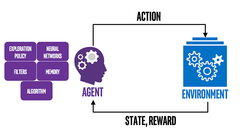
The Agent & Environment:
Imagine teaching a dog a new trick. You give commands, and the dog performs actions. If it does well, it gets a treat; if it doesn’t, it gets no reward or even a slight reprimand. In RL:
- Agent: The learner or decision-maker, akin to the dog.
- Environment: Everything the agent interacts with, which, in our analogy, includes you, the command, and the surroundings.
The agent takes actions in the environment, which then transitions to a new state and returns rewards as feedback to the agent.
State, Action, and Reward:
- State (s): The current scenario or situation the agent finds itself in.
- Action (a): The decisions or moves made by the agent in response to a state.
- Reward (r): The feedback the agent receives after acting in a state. It’s the agent’s immediate measure of how good or bad the action was.
Policy:
The policy is the agent’s strategy to determine the following action based on the current state. It can be deterministic (a direct mapping from state to action) or stochastic (giving probabilities of choosing various actions).
Value Functions:
- Value Function (V(s)): Represents the expected long-term reward with a discount for a given state. It tells us the worth of a state.
- Q-function (Q(s, a)): Represents the expected return of taking action in state s. This is pivotal for many RL algorithms, allowing the agent to evaluate each action in a given state.
Exploration vs. Exploitation Dilemma:
In the process of learning, an agent faces a fundamental challenge:
- Exploration: Trying new actions to discover their effects.
- Exploitation: Using known actions that yield the highest rewards.
Striking a balance is crucial. Too much exploration can result in unnecessary risks, while excessive exploitation can lead to missed opportunities.
Discount Factor:
The discount factor (γ) determines the present value of future rewards. A value of 0 makes the agent short-sighted, focusing only on immediate rewards, while a value close to 1 makes the agent prioritize long-term rewards.
Model-based vs. Model-free:
- Model-based: These methods try to predict what the environment will do next. It’s like playing chess and trying to anticipate your opponent’s moves.
- Model-free: These methods don’t care about the environment’s model. Instead, they focus on learning the value function or policy directly from experiences.
Learning Methods:
- Off-Policy: The agent learns the value of the optimal policy independently of the agent’s actions, e.g., Q-learning.
- On-Policy: The agent learns the value of the policy being carried out by the agent, e.g., SARSA.
What is Q-learning?
Q-learning is a model-free, off-policy RL algorithm that seeks to find the best action-selection policy for a given finite Markov decision process. It helps agents find the optimal strategy (or action) in every situation (or state) to achieve the maximum cumulative reward over time.
The Building Blocks of Q-learning
Q-table:
The heart of Q-learning lies in the Q-table, a matrix where rows represent states and columns represent possible actions. The value in each cell (denoted as Q(s, a)) represents the expected future reward for taking action an in state s.
Bellman Equation:
Q-learning employs the Bellman equation to update Q-values:
Q(s,a)=(1−α)×Q(s,a)+α×(r+γ×maxa′Q(s′,a′))Q(s,a)=(1−α)×Q(s,a)+α×(r+γ×maxa′ Q(s′,a′))
Where:
- αα is the learning rate, determining to what extent new Q-values are adopted.
- γγ is the discount factor, capturing the importance of future rewards.
- rr is the immediate reward after taking action in state s.
- maxa′Q(s′,a′)maxa′ Q(s′,a′) is the highest Q-value for next state s′s′.
Exploration vs. Exploitation:
For Q-learning to be effective, the agent must explore enough to understand its environment and exploit its knowledge to maximize rewards. This is typically managed by the ε-greedy strategy, where the agent occasionally tries a random action (exploration) but mostly chooses the action with the highest Q-value (exploitation).
The Q-learning Algorithm:
- Initialization: Start with a Q-table filled with zeros.
- Exploration: For each episode (or trial), the agent explores its environment. In each state, it can choose an action based on a policy derived from the current Q-value, often with some randomness to encourage exploration.
- Learning: After taking an action and receiving a reward from the environment, the Q-value of the action taken in the current state is updated using the Bellman equation.
- Repeat: Continue exploring and learning until a termination condition is met, such as a maximum number of episodes or minimal changes in Q-values.
Step-by-Step Implementation:
Let’s use the Q-learning algorithm (a model-free, off-policy RL algorithm) to train an agent on the FrozenLake environment from the gym, a widely-used RL library.
1. Install the necessary libraries:
pip install gym numpy2. Import the libraries and initialize the environment:
import numpy as np
import gym
env = gym.make('FrozenLake-v0', is_slippery=False)
3. Initialize the Q-table:
state_space_size = env.observation_space.n
action_space_size = env.action_space.n
q_table = np.zeros((state_space_size, action_space_size))
4. Set hyperparameters:
alpha = 0.1  # Learning rate
gamma = 0.99  # Discount factor
epsilon = 1.0  # Exploration rate
epsilon_decay = 0.995
epsilon_min = 0.01
num_episodes = 10000
5. Q-learning Algorithm:
for episode in range(num_episodes):
    state = env.reset()
    done = False
while not done:
if np.random.uniform(0, 1) < epsilon:
action = env.action_space.sample() # Explore
else:
action = np.argmax(q_table[state, :]) # Exploitnew_state, reward, done, _ = env.step(action)# Update Q-values using the Bellman equation
q_table[state, action] = q_table[state, action] + alpha * (reward + gamma * np.max(q_table[new_state, :]) - q_table[state, action])
state = new_state# Decay epsilon
if epsilon > epsilon_min:
epsilon *= epsilon_decay
6. Test the trained agent:
num_test_episodes = 10
for episode in range(num_test_episodes):
    state = env.reset()
    done = False
    print("Episode", episode+1)
    while not done:
        env.render()
        action = np.argmax(q_table[state, :])
        state, _, done, _ = env.step(action)
    env.render()
Following this guide, you can set up a simple reinforcement learning experiment using Q-learning in the FrozenLake environment. As you advance, consider exploring more complex algorithms like DDPG, A3C, and PPO, and use libraries like TensorFlow or PyTorch for more advanced RL applications.
Stay tuned, and happy coding!
Visit my Blog for more articles, news, and software engineering stuff!
Follow me on Medium, LinkedIn, and Twitter.
All the best,
CTO | Tech Lead | Senior Software Engineer | Cloud Solutions Architect | Rust 🦀 | Golang | Java | ML AI & Statistics | Web3 & Blockchain
#reinforcementlearning #openaigym #rlenvironments #rlresearch #gymtutorial #rltools #classiccontrol #toytext #atari #robotics #gymbenchmarking #quickprototyping
