Building a Machine Learning Model from Scratch Using Python
Machine Learning (ML) models allow us to make predictions, identify patterns, and even make data-based decisions.

Machine Learning (ML) models allow us to make predictions, identify patterns, and even make data-based decisions.
In this article, we will build a simple linear regression model from scratch using Python.
1. Define the Problem
Before diving into the code, clearly define the problem you want to solve. For this guide, we’ll use linear regression to predict a continuous value. Specifically, let’s predict house prices based on a single feature: house size.
2. Gather Data
For our example, let’s assume we have a dataset with two columns: House Size (in square feet) and House Price.
data = {
    'size': [650, 785, 1200, 1400, 1800],
    'price': [77250, 92850, 150000, 178000, 215000]
}
3. Prepare Data
Most of the time, data will require preprocessing, such as normalisation, dealing with missing values, or encoding categorical variables. For simplicity, we’ll normalise our data using Min-Max scaling:
def normalize(values):
    min_val = min(values)
    max_val = max(values)
    return [(v - min_val) / (max_val - min_val) for v in values]

data['size'] = normalize(data['size'])
data['price'] = normalize(data['price'])
4. Build the Model
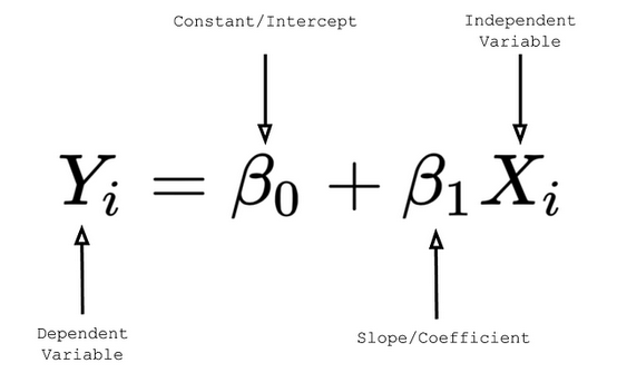
We’ll use the simple linear regression formula:

Where:
- Y is the dependent variable (house price in our case).
- X is the independent variable (house size).
- m is the slope of the line.
- b is the y-intercept.
Initialize parameters:
m = 0
b = 0
learning_rate = 0.01
epochs = 1000
Cost Function:
We use the Mean Squared Error (MSE) as our cost function. The Mean Squared Error (MSE) is a commonly used metric to measure the average squared difference between actual and predicted values in regression problems. It helps to quantify the accuracy of a model in predicting continuous values.
The formula for MSE is:

Where:
- Y is the actual value for the i-thith observation.
- Y^ is the predicted value for the i-thith observation.
- n is the total number of observations or data points.
def compute_cost(m, b, data):
    total_cost = 0
    N = len(data['size'])

    for i in range(N):
        x = data['size'][i]
        y = data['price'][i]
        total_cost += (y - (m*x + b)) ** 2

    return total_cost / N
Gradient Descent
Gradient Descent is an optimisation algorithm commonly used to minimise (or maximise) a function iteratively. It’s trendy for training machine learning models, especially in the context of deep learning and neural networks.
The main idea behind gradient descent is to update the parameters of a model iteratively to minimise a cost or loss function.
Here’s a high-level explanation:
- Initialisation: Choose an initial set of parameters (often randomly).
- Compute the Gradient: For the current set of parameters, compute the gradient of the cost function. The gradient is a multi-dimensional derivative that points in the direction of the steepest ascent. Since we want to minimise the function, we will move in the direction opposite to the gradient.
- Update the Parameters: Adjust the parameters toward the negative gradient. This step size is controlled by a parameter called the learning rate. A high learning rate might make the optimisation jump over minima, while a meagre learning rate might slow the optimisation process.
- Iterate: Repeat steps 2 and 3 until the gradient is very close to zero (i.e., you’ve reached a minimum) or until a predetermined number of iterations have been reached.
Implementation:
def gradient_descent(m, b, data, learning_rate):
    m_gradient = 0
    b_gradient = 0
    N = len(data['size'])

for i in range(N):
        x = data['size'][i]
        y = data['price'][i]
        m_gradient += -2/N * x * (y - (m*x + b))
        b_gradient += -2/N * (y - (m*x + b))
    m = m - learning_rate * m_gradient
    b = b - learning_rate * b_gradient
    return m, b
Training:
for epoch in range(epochs):
    m, b = gradient_descent(m, b, data, learning_rate)
    if epoch % 100 == 0:
        print(f"Epoch {epoch}, Cost: {compute_cost(m, b, data)}, m: {m}, b: {b}")
5. Evaluate the Model
We can use the MSE cost we defined earlier to evaluate the model. In a real-world scenario, you’d split your data into training and testing datasets to assess the model’s performance on unseen data.
6. Make Predictions
With the trained model, we can make predictions:
def predict(m, b, x):
    return m * x + b

# Predicting price for a normalized house size (for demonstration purposes)
normalized_size = (1000 - 650) / (1800 - 650)  # Assuming a house size of 1000 sq ft

predicted_price = predict(m, b, normalized_size)

print(f"Predicted normalized price for house size of 1000 sq ft: {predicted_price}")
Run the code above to build the linear regression model, train it using gradient descent, and make a prediction for a house size of 1000 sq ft. Adjust learning_rate and epochs as needed to ensure convergence.
Building a machine learning model from scratch offers a deep understanding of the underlying mathematics and algorithms. While this benefits educational purposes, you’d often leverage libraries like scikit-learn or TensorFlow, which provide optimised and extended functionality.
Nevertheless, grasping the fundamentals by creating simple models from scratch is an invaluable learning experience for anyone diving into machine learning.
Stay tuned, and happy coding!
Visit my Blog for more articles, news, and software engineering stuff!
Follow me on Medium, LinkedIn, and Twitter.
All the best,
CTO | Senior Software Engineer | Tech Lead | AWS Solutions Architect | Rust | Golang | Java | ML AI & Statistics | Web3 & Blockchain
#MachineLearningBasics #PythonProgramming #LinearRegression #DataScience #MLFromScratch #DataPreprocessing #GradientDescent #PredictiveModeling #AI #DeepLearning #DataAnalysis #TechTutorial #ModelTraining #MLAlgorithms


